analisis teknikal IHSG dengan python - labs127.io and me
Skrip1 ini pertama kali saya buat tahun 2013 yang lalu, dan baru saja diperbarui, menyesuaikan dengan beberapa dependencies yang sudah berganti versi. Gambaran skrip ini sebagai berikut:
- ambil data dari yahoo finance2
- olah data dengan
pandas3 - gambar plot dengan
matplotlib4 - update twitter dengan
twython5
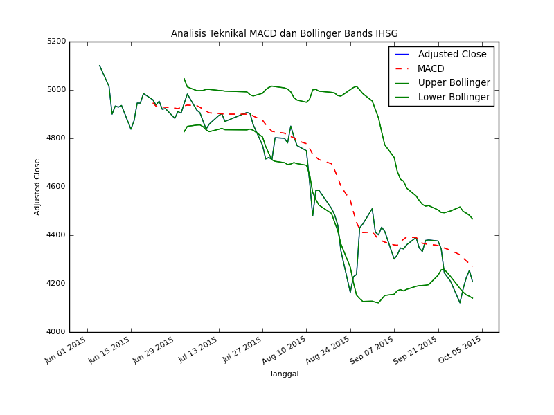
Hasil analisis teknikal ini dapat dibaca sebagai berikut:
Jika harga adjusted close (garis tengah tidak putus) menyentuh garis upper bollinger band, maka ini merupakan sinyal jual. Dan sebaliknya, jika harga adjusted close, menyentuh garis lower bollinger band, maka ini berarti sinyal untuk beli.
# app.py
from twython import Twython
import pandasaham as pshm
import time
import datetime

now_time = datetime.datetime.fromtimestamp(
    time.mktime(time.gmtime(
        (datetime.datetime.utcnow() - datetime.datetime(1970, 1, 1)) \
        .total_seconds() + 25200))).strftime('%Y-%m-%d %H:%M:%S')

# url
# https://twython.readthedocs.org/en/latest/usage/advanced_usage.html

cons_key = ''
cons_secret = ''
acc_token = ''
acc_token_sec = ''

t = Twython(app_key=cons_key,
            app_secret=cons_secret,
            oauth_token=acc_token,
            oauth_token_secret=acc_token_sec)


# download and analyze it
pshm.dl()
# update twitter _with_media
photo = open('ihsg.png', 'rb')
t.upload_media(status='[Autotwit] Grafik Pergerakan IHSG 3 bulan terakhir ' \
               'dgn Analisis MACD ' + now_time + ' #saham #ihsg #jci #idx',
               media=photo)
photo.close()
# pandasaham.py
import pandas as pd
import matplotlib
import matplotlib.pyplot as plt
import numpy as np
from datetime import datetime, timedelta
import re
import time
import urllib2

# download data
def dl():
    url = 'http://finance.yahoo.com/q/hp?s=%5EJKSE+Historical+Prices'
    html = urllib2.urlopen(url).read()
    pattern = re.compile(r"http://real-chart.*=\.csv\"")
    m = re.search(pattern, html).group()

    with open('table.csv', 'wb') as f:
        f.write(urllib2.urlopen(m).read())

    df = pd.read_csv('table.csv', index_col='Date', parse_dates=True)
    df = df.sort_index(ascending=True)
    df = df.tail(80)
    # analysis
    macd = pd.rolling_mean(df['Adj Close'], 12)
    # bollinger bands
    # https://github.com/arvindevo/MachineLearningForTrading/blob/master/bollingerbands.py
    movavg = pd.rolling_mean(df['Adj Close'], 20, min_periods=20)
    movstddev = pd.rolling_std(df['Adj Close'], 20, min_periods=20)
    upperband = movavg + 2*movstddev
    lowerband = movavg - 2*movstddev

    # plot settings
    matplotlib.rcParams.update({'font.size': 8})
    s = datetime.now()

    # begin plot
    df['Adj Close'].plot(label='Close')
    macd.plot(label='macd', linestyle='--', color='r')
    upperband.plot(color='green')
    lowerband.plot(color='green')

    plt.title('Analisis Teknikal MACD dan Bollinger Bands IHSG')
    plt.legend(['Adjusted Close', 'MACD', 'Upper Bollinger', 'Lower Bollinger'])
    plt.xlim(s - timedelta(days=130), s + timedelta(days=7))
    plt.ylabel('Adjusted Close')
    plt.xlabel('Tanggal')

    # save the image for twitter update with image
    plt.savefig('ihsg.png')

    # show graph
    # plt.show()

dl()